
Correlation in a portfolio is a number, usually between -1 and +1, that shows how closely two investments move in the same direction over the same period. It tells you whether holding something beside your main asset spreads risk or quietly doubles it. A value near +1 means the two move in lockstep, near 0 means they move independently, and near -1 means they tend to move in opposite directions. That single figure is what separates real diversification from owning the same bet several times over.
Most self-directed investors meet the phrase in a diversification lecture and never see it again. It stays abstract, so it never changes a decision. The intention of this guide is to make it concrete: what the coefficient measures, what a decent number looks like, and how to run the check on your own holdings this weekend without any paid tool.
Nothing here is personalised advice. Correlation is a statistical description of past behaviour, useful for thinking about risk, and useless as a prediction of what happens next.
Table of Contents
- What Is Correlation in a Portfolio?
- How Is Portfolio Correlation Calculated?
- The formula in plain English
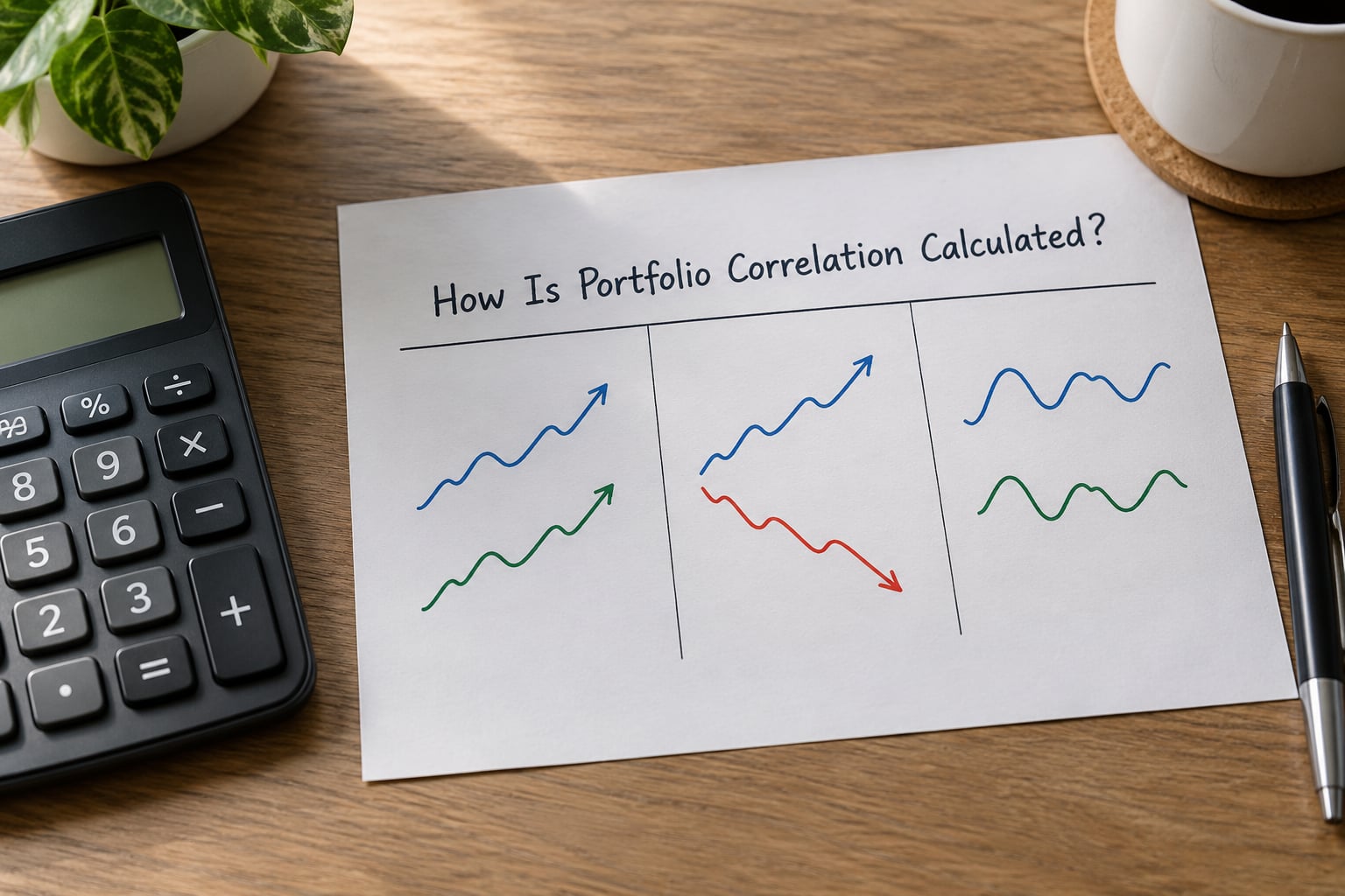
- What the coefficient values mean
- Choosing a sample window
- Rolling correlation versus one fixed number
- What Do Positive and Negative Correlations Mean?
- How Does Correlation Affect Diversification?
- What Is a Good Correlation Level for a Portfolio?
- How Can Investors Use Correlation When Building a Portfolio?
- What Are the Limitations of Correlation?
- Frequently Asked Questions
- What is the ideal correlation for a portfolio?
- What does correlation mean in simple terms?
- Is a correlation of 0.7 considered diversified?
- Why do correlations increase during a market crash?
- How many assets do I need in a diversified portfolio?
- How do I calculate the correlation between two stocks?
- Conclusion
What Is Correlation in a Portfolio?
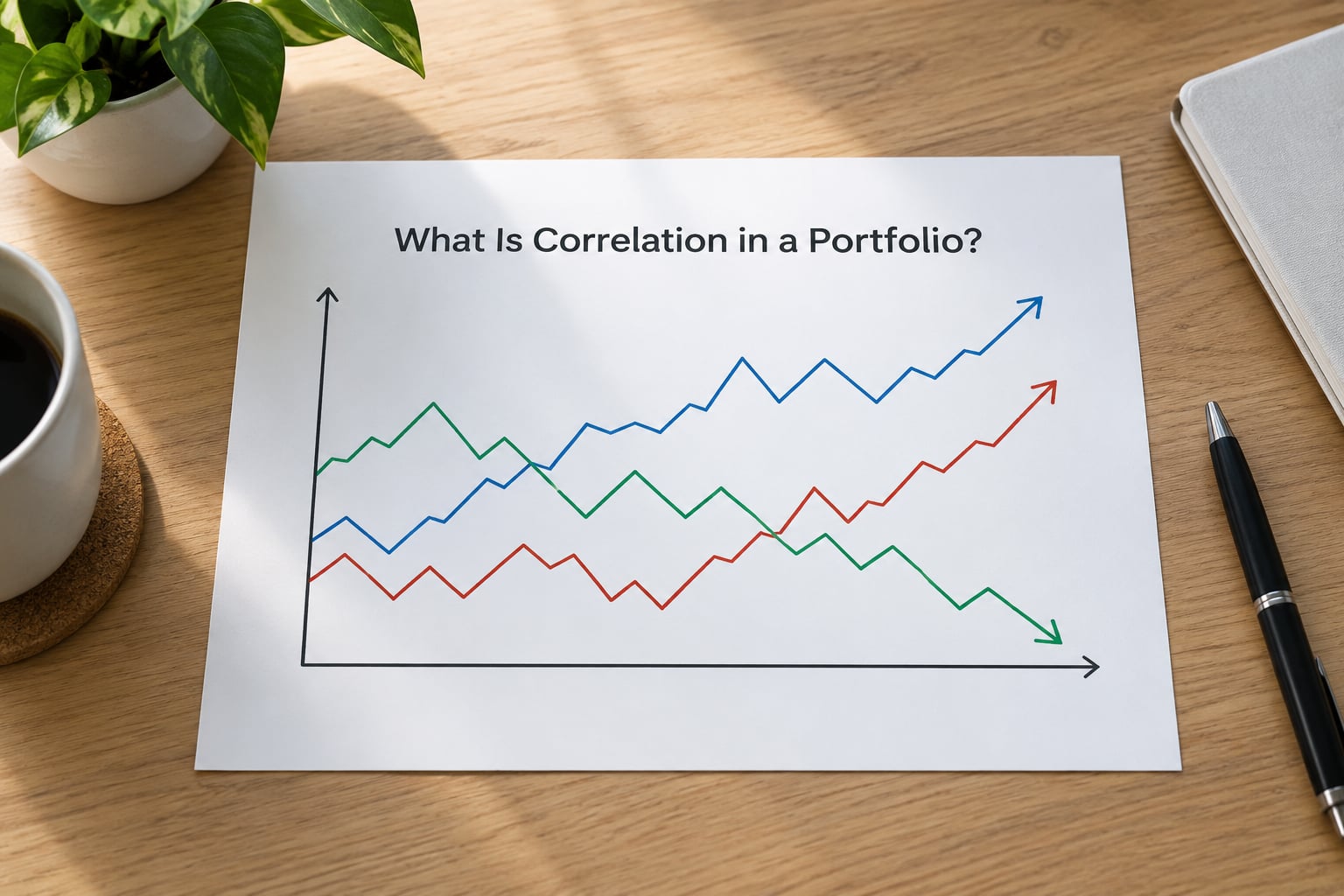
Correlation in a portfolio measures how closely the returns of two or more assets move together over a chosen period, expressed as a coefficient between -1 and +1. It captures the relationship between holdings, not the performance of any single holding, and it is the reason a portfolio can be less risky than the average of the assets inside it.
That last point trips people up, so it is worth being slow here. Each asset on its own has its own volatility, which is simply how far its returns bounce around its average, measured as standard deviation. Correlation says nothing about that. It only describes the pattern of the moves themselves: do the up months and down months line up, partly line up, or line up in reverse.
Two funds can each be volatile and still combine into something calmer than either one alone, purely because they wobble at different times. A third fund that rises and falls almost exactly with the first adds no new risk structure at all, no matter what its name suggests.
Put plainly, diversification means holding assets that are not correlated with one another. That reframes what diversification actually is: it is about counting distinct risks rather than counting positions, since two portfolios of ten holdings each can behave completely differently.
How Is Portfolio Correlation Calculated?
The formula in plain English
The calculation starts by converting prices into returns, because prices on very different scales cannot be compared directly. Take the percentage change in each asset for every period in your sample, then measure how closely those two series of numbers move together.
The correlation coefficient, usually written as r, is the average of the products of each asset’s deviation from its own mean, divided by the product of their standard deviations. Written out, it looks like this:
r = SUM( (return A minus its mean) x (return B minus its mean) ) divided by the square root of SUM(return A minus its mean squared) x SUM(return B minus its mean squared)
You do not need to do this by hand. In a spreadsheet, two columns of periodic returns and the function =CORREL(A2:A121, B2:B121) gives you the number, and filling the function across a grid of columns produces the correlation matrix most portfolio tools display.
What the coefficient values mean
Here is the scale in one place. The example pairs are illustrative, drawn from the way broad asset classes have typically behaved rather than from any live data.
| Coefficient | Plain-English meaning | Effect on portfolio risk | Typical example pair |
|---|---|---|---|
| +1.0 | Perfectly positively correlated; the two move in exact proportion | No diversification benefit whatsoever | Two funds tracking the same large-cap index |
| +0.7 to +0.9 | Strongly correlated | Adds holdings without meaningfully adding different risk | A global large-cap fund and a domestic large-cap fund |
| +0.3 to +0.6 | Moderately correlated | Some risk reduction, less than you would expect | US equities and UK equities |
| 0.0 to +0.2 | Weak or near-zero relationship | Meaningful diversification benefit | Equities and short-dated government bonds |
| -0.1 to -0.4 | Weakly negatively correlated | Strong benefit; tends to cushion the combination | Equities and gold over some periods |
| -1.0 | Perfectly inversely related; one rises exactly as the other falls | Hedging in principle, and effectively impossible in real markets | Theoretical; treat any real -1 as a data error |
Choosing a sample window
Correlation is only ever measured over a window you picked, which makes it far more fragile than it looks. Daily returns over three years and monthly returns over fifteen years can produce noticeably different numbers for the same pair of assets, and neither is wrong, because they are answering different questions.
Most published studies run a decade or more of monthly data for broad asset classes and five years or more of daily data for individual funds. Any figure you meet without a stated window deserves a follow-up question.
Rolling correlation versus one fixed number
A rolling correlation recomputes the coefficient over a sliding window, so each point reflects only the most recent stretch of history. It is the more honest presentation, because it shows the relationship drifting instead of pretending a single number describes the whole period.
Look for a chart of rolling correlation between your two assets rather than a headline figure. A pair that averaged +0.35 across a decade might have spent the last two years above +0.8, which is a very different portfolio to be holding today.
What Do Positive and Negative Correlations Mean?
Positive correlation simply means the two assets tend to rise and fall together, and it is by far the most common relationship in a typical account. Two large-cap equity funds, even from different providers, usually sit well above +0.8 with each other.
A correlation of exactly +1 means the two move in the same direction and in the same proportion, every period. That is what two funds tracking the identical index produce, which is why owning both halves your position size while leaving your risk almost unchanged. The everyday version of this is buying two different large-cap funds and assuming you own two things, when the second is quietly the first one again.
A correlation of 0 means no measurable relationship in either direction. The assets move independently as far as the data can tell. Independent movements are what make a combination genuinely steadier, because gains in one can offset losses in the other by chance rather than by design.
Negative correlation means the two tend to move in opposite directions. Gold against equities is the example most often given, though the strength of that relationship shifts with interest rates and with how frightened markets happen to be. A perfectly negative correlation of -1 is a mathematical nicety rather than something you will meet in a real account.
Cash is the one reliable low-volatility asset in most portfolios, and it does not so much offset equity losses as stop fresh money from adding to them during a bad stretch. Commodities, including precious metals, are usually discussed as diversifiers for the same reason: their drivers, such as inflation expectations and currency swings, are not the same as the earnings revisions that drive equity prices.
For orientation, here are typical ranges between broad asset classes. Treat these as illustrative rather than current, and recheck them against recent data for your own market.
| Asset pair | Illustrative range | Comment |
|---|---|---|
| Global equities vs domestic equities | +0.6 to +0.9 | Different listings, largely the same underlying companies |
| Large-cap growth vs small-cap value | +0.7 to +0.9 | Style differences barely separate them in a downturn |
| Equities vs government bonds | -0.2 to +0.4 | The sign itself has flipped across different eras |
| Equities vs gold | -0.3 to +0.3 | Often low, occasionally clearly negative, never stable |
| Equities vs cash | Close to 0 | Cash barely moves, so there is little to co-move with |
How Does Correlation Affect Diversification?
Here is where the coefficient earns its place, using an illustrative two-asset example. Take two holdings, one with 15% annual volatility and one with 8%, held in equal weight. Nothing about the calculation is a forecast; it only shows what the correlation coefficient does to the combined result.
| Correlation between the two | Combined portfolio volatility | What it means |
|---|---|---|
| +1.0 | 13.9% | No benefit; the portfolio is just as bumpy as its parts |
| +0.5 | 11.5% | Modest reduction, equal to the weighted average of the parts |
| +0.2 | 9.8% | Clear reduction, roughly 30% below the weighted average |
| -0.5 | 3.5% | Dramatic smoothing, because the two offset each other |
The weighted average of those two holdings’ volatilities is 11.5%, so you only beat it once correlation drops below roughly 0.5. That is the practical heart of diversification: the benefit comes from the relationship between holdings, not from the count of them.
Now a three-asset version, which is closer to a real account. Suppose 50% in equities with 15% volatility, 30% in bonds with 8% volatility and 20% in gold with 14% volatility. Pair them with equities and bonds at +0.2, equities and gold at -0.1, and bonds and gold at +0.4.
Run those figures through the portfolio variance formula and the result is roughly 8.8% volatility. The weighted average of the individual volatilities is 12.7%. The portfolio is meaningfully calmer than its parts despite holding a fairly aggressive-looking mix, and almost all of that comes from the pair relationships rather than from the asset labels.
Weight matters as much as the coefficient. Two holdings at 90% and 10% produce far less diversification than two holdings at 50% and 50%, even with an identical correlation. Sizing is what turns a decent pair of numbers into a portfolio that behaves the way you expected.
What Is a Good Correlation Level for a Portfolio?
There is no ideal correlation for a portfolio, only pair relationships and trade-offs. If you are asking what number to aim for, broadly below +0.3 between your main risk drivers is where the diversification benefit starts to be real, and genuinely negative correlation is the ideal but stays rare in practice.
Above roughly +0.7, two holdings are largely redundant. Holding both is a decision about position size and provider preference rather than about diversification. That threshold is a rule of thumb, not a law, and it is worth checking against your own data rather than taking it from anyone.
| Level | Reading in practice | Action |
|---|---|---|
| Below 0.2 | Nearly independent | Keep the pairing, it is doing real work |
| 0.2 to 0.4 | Useful partial diversification | Reasonable as a core pairing |
| 0.4 to 0.6 | Weak benefit only | Check whether the pair earns its place |
| 0.6 to 0.8 | Largely redundant | Look for a different source of exposure |
| Above 0.8 | The same bet twice | Consolidate, unless you are sizing deliberately |
Because correlation is a relationship and not a portfolio-level score, the number to watch is usually the average of your holdings’ correlations with each other. A portfolio where everything sits between +0.5 and +0.7 is thinly diversified, however many line items it shows on screen.
How Can Investors Use Correlation When Building a Portfolio?
Running the check yourself takes about an hour and no software beyond a spreadsheet. If you have never done it, the practical answer to what is correlation in a portfolio at the holdings level is a matrix of pairwise coefficients between your positions, built from periodic returns.
- List your holdings and weights. Start with your largest positions, since a small holding barely moves the pair relationships that matter. Include cash, since it counts as a position with its own behaviour.
- Get periodic returns for each. Export monthly returns over five to ten years from whatever provider you use, or take closing prices and convert them to percentage changes yourself. Use the same frequency for every asset, and check for missing data before you start.
- Compute the matrix. In a spreadsheet, use =CORREL() for each pair and lay the results out in a grid. Read the rows, not just the average. One alarming number matters more than a flattering overall figure.
- Check for hidden overlap. For funds and ETFs, look at the underlying holdings rather than the fund names. Two products tracking similar indices will show a correlation near +1 even when their labels and objectives read differently, and paying an active fee on top of index-like exposure is a particularly expensive version of that mistake.
- Recheck periodically. A rolling correlation chart, refreshed a few times a year, tells you when a relationship has drifted far enough to matter. Put the review on a schedule rather than waiting for a dramatic drop.
On the number of holdings question that runs through the beginner forums, correlation gives a better answer than counting does. A portfolio holding 43 stocks across 11 sectors plus ETFs often reads as diluted on screen, and that reaction is usually a sign of near-perfect correlation across the holdings rather than genuine breadth. Count distinct sources of risk instead.
There is also a formal version of this idea. Modern portfolio theory uses the correlation matrix to construct a minimum variance portfolio, and risk parity goes further by setting position sizes to equalise each holding’s contribution to risk rather than its share of capital. Neither is something you need in order to build a sensible mix, but they are the names to search for if you want the theory behind the numbers above.
What Are the Limitations of Correlation?
Correlation is a backward-looking statistic, and that single limitation explains most of the others. It summarises what two assets did together in a chosen window; it says nothing about what they will do next, and a relationship that held for a decade can break over a quarter.
Correlations also tend to rise toward +1 during market stress, which is exactly when diversification is most needed. In a sharp sell-off, investors sell what they can, and assets that behaved independently in calm markets start falling together. The diversification that looked real on a chart can be largely unavailable in the week you need it.
Regime changes cause the same problem more slowly. Interest rate environments, inflation regimes and shifts in market structure all reshape pair relationships, and a coefficient measured across several different regimes can be an average of behaviours that have little in common.
Data choices matter too. Different return frequencies, different time zones for daily closes, distributions that are treated as income rather than price moves, and survivorship bias in funds that have merged can all shift a result without anything being wrong.
Finally, correlation measures co-movement, not risk in full. A pair with a correlation of +0.1 can still be exposed to the same single event, such as a rate decision or a commodity shock, and that shared exposure will not appear in any number. It is also worth keeping it distinct from the three terms beginners mix up with it.
| Term | What it measures | Scale | How it differs from correlation |
|---|---|---|---|
| Correlation | Direction and strength of co-movement between two return series | -1 to +1 | The relationship itself |
| Covariance | The same co-movement in raw units of return multiplied by return | Unbounded, units change with the assets | Correlation is covariance divided by the two standard deviations, which is what makes it comparable across asset pairs |
| Standard deviation | How widely a single asset’s returns scatter around their average | Percentage points | Describes one asset, not a relationship |
| Beta | How far an asset moves relative to a chosen benchmark | Typically around 1 | Compares an asset with a market, so it mixes direction with sensitivity rather than isolating direction alone |
If you take one caution from all of this, make it the first one: a correlation number describes a past sample, useful for spotting redundancy and for thinking about how positions might interact, and never a forecast.
Frequently Asked Questions
What is the ideal correlation for a portfolio?
There is no single ideal figure, but broadly below +0.3 between your main risk drivers is where diversification starts to do real work, and negative correlation is the ideal that rarely holds. Above roughly +0.7, two holdings are largely redundant, because the second adds position size rather than a different risk profile. Treat these as rule-of-thumb thresholds and check them against your own data.
What does correlation mean in simple terms?
Correlation means how closely two investments move together. A value of +1 means they rise and fall in lockstep, 0 means they move independently with no clear link, and -1 means they tend to move in opposite directions. The point of measuring it is simple: assets that do not move together smooth out each other’s bad periods, and assets that do move together just repeat the same risk.
Is a correlation of 0.7 considered diversified?
Not really. At +0.7 the two holdings share most of their ups and downs, so holding both gives you more position size rather than a genuinely different exposure. For reference, the combined volatility of two equally weighted assets with 15% and 8% individual volatility is 11.5% at a +0.5 correlation but about 9.8% at +0.2. Below +0.3 the benefit becomes material.
Why do correlations increase during a market crash?
During a sell-off, investors sell what they can and buyers step away, so assets that moved independently in calm markets start falling together. Cash flows that are usually independent, such as fund redemptions, become correlated pressure during forced selling. This is why diversification benefit tends to shrink at the worst possible moment, and why a long-run average coefficient can overstate the protection available in a crisis.
How many assets do I need in a diversified portfolio?
There is no number, because holdings that move together count as one risk no matter how many line items they occupy. The better test is the correlation between your positions: if most pairs sit below +0.3, a moderate number of holdings is doing useful work. Forty holdings drawn from the same index are one holding. Count distinct sources of return and risk rather than positions.
How do I calculate the correlation between two stocks?
Collect periodic returns for both stocks over the same window, such as monthly returns over five years, then run =CORREL() on the two columns in a spreadsheet. The result is a coefficient between -1 and +1. Check the window and the frequency you used, and prefer a rolling correlation chart over a single number, since the relationship between two stocks can shift substantially over a few years.
Conclusion
Start where the work is highest. List your largest holdings, run a CORREL check across them, and look for pairs above +0.7 that are quietly the same investment twice. That single exercise tells you more about whether you are diversified than any number of accounts or line items does.
What is correlation in a portfolio, in the end? It is a backward-looking measure of whether your holdings actually do different jobs. Use it to find redundant risk, to size positions honestly, and to know that the relationship you measured last year is not guaranteed to hold through the next one.